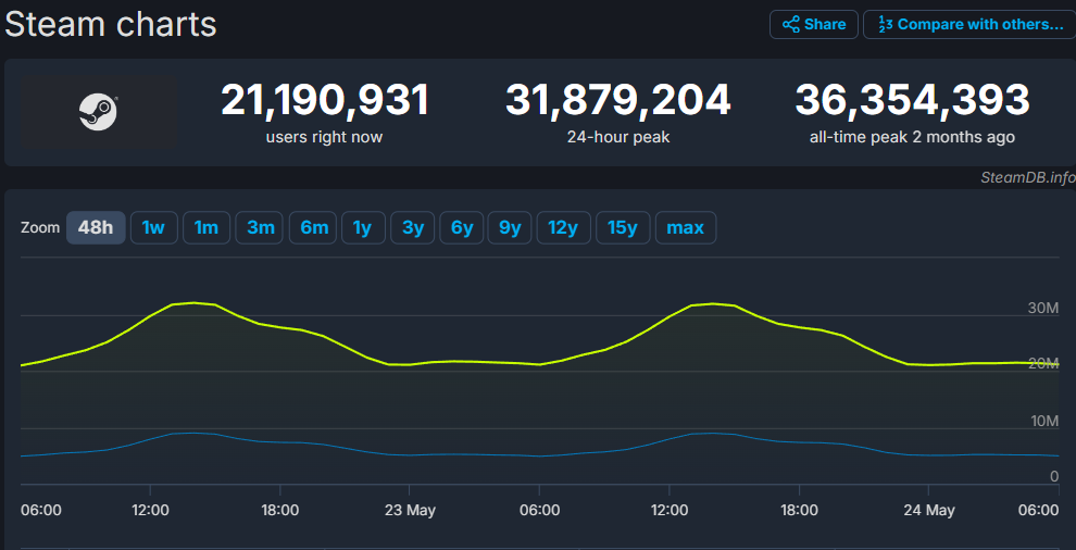
Online gaming platform Steam, is one of the most popular computer platforms for players to connect online with one another and download the latest digital releases of games.
SteamDB, an unaffiliated third-party website, collects Steam related data and was created to provide insights into the official Steam database. The company has collected the records of Steam’s player counts, including the number of in-game active users, from January 2013 to October 2022.
Using these records, we provide a useful forecast into the number of active users, for use by the Steam management team to gain a better understanding of the necessary equipment required to handle their expected server usage for the coming terms.
Some assumptions made in the process of this project include the general assumption that SteamDB has collected this data accurately and that it is well maintained. Additionally, we need to assume that the data collected by SteamDB is truly representative of the official Steam database.
The time series data in this report is used to analyze the pattern in the daily user count for the Steam platform. We could conclude that there is a strong seasonality in daily active users on Steam, and the period time is seven days. We created a seasonal ARIMA model that could forecast an estimate of the number of future active players
01 Introduction
There are roughly 3.2 billion gamers worldwide, easily earning gaming the reputation of being the single most popular hobby around the world. This accounts for approximately 40% of the entire population.
As this may be hard to believe, gaming has become a very mainstream form of entertainment and is constantly growing in accessibility. With a very diverse set of devices to play on, ranging from consoles, to computers, to smartphones, the industry has become bigger than the music and movie industries in earnings combined.
The most popular gaming device is the PC, with a substantial 1.7 billion gamers. Steam is the leading online game distribution platform for PC, raking in massive business from the commission of game purchases, rentals, in-game add-ons, downloadable content, licensing fees and more. As the lead platform in the industry, there is massive server usage with maintenance required to hold its top spot in this sector.
The data we will be working with has been collected by SteamDB, an unaffiliated third-party, collecting Steam data by using a combination of data mining, web scraping, and APIs made publicly available from Steam itself. This data can give us a very useful insight into the true server usage statistics of the official Steam database. The data set consists of the daily user counts from 2004 to 2022, and began recording the number of active users in 2017.
02 Objectives
Using this data, we plan to analyze the number of gamers using the Steam platform to gain a deeper understanding of the correlation and response that is happening between concurrent daily player counts.
Using this understanding, we will attempt to fit the best model from what we have learned throughout the course and apply it to the series using the R statistical software. Once a sufficient model is fit, we use it for forecasting in order to provide Steam with a rough estimate of their server usage for the following 6 months to a year.
Additionally, a good understanding of the type of model fit can help us to study extreme events and use it to determine probable shocks during this time.
03 Analysis
3.1 Preporcesssing
We read the data into R and stored the data into a variable named steam.raw using the function read.csv below,
> steam.raw <- read.csv("chart.csv", header=True)setting the header parameter to TRUE in order to use the header line of the csv file as column names. Upon examining the data, we found that there are four recorded variables: DateTime, Users, In.Game, and Flags. We also found that the variable Flags is completely missing its values, and In.Game is missing roughly 73% of its values.
> colMeans(is.na(steam.raw))>>> DateTime Users In.Game Flags
0.00000000 0.06275304 0.73279352 1.00000000Considering the missing observations for Flag, we choose to omit this variable. The high percentage of missing values in In.Game is not alarming as the majority of these values are from before 2017.
However, even if we were to use data from 2017 and on, there are a few gaps left in this time series. Records from March 21, 2017 to March 22, 2017, February 21, 2018 to February 25, 2018 and February 18, 2019 to February 19, 2019 all have missing observations.
These unreported values may be the results of technical errors in the data collection process. We thought about replacing the NAs with zeros, as there may have been a server outage for these dates. However, this will greatly alter the original distribution of the dataset by reducing the mean E(Y).
We then thought about imputing the NAs with E(Y), but this may also change the distribution of the original data. Thus, we only keep records from 2020 and on such that we are left with a continuous time series.
3.2 Assumptions
The cleaned time series keeps the data recent, and relevant to the server capabilities of today’s technology, however, in using this data we need to make some assumptions about its integrity.
We assume that the Steam data provided by SteamDB has been collected accurately, and that it is well maintained. We also need to assume that the data is truly representative of the official Steam database in order to make any conclusions about Steam’s server usage.
Ourforecast will be a rough approximation because of this, however, if Steam were truly interested in our findings, we could use our analysis to fit a model on the true data, given their consent.
Finally, we decide to further exclude data from before 2020 in our analysis of the cleaned data, to reduce the effects of covid-19 on the number of in-game Steam players.
3.3 Trends
The visual trend of the data is a gradual positive increase of In.Game players over time. By the look of the series, we can make the conjecture that the series may be of the moving average model type, given its shape.
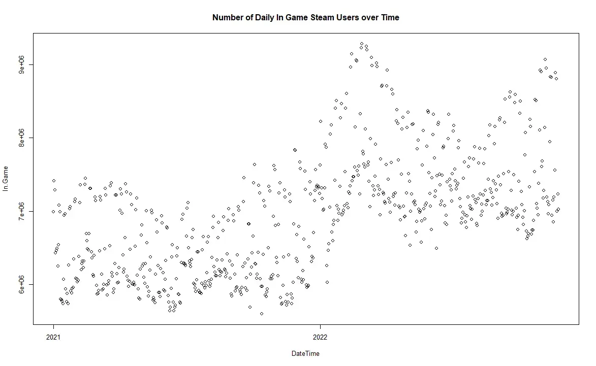
There also appears to be some annual seasonality happening with the number of in-game players, however, we will touch on this later. We now begin our model fitting using the Box-Jenkins approach.
3.4 Box-Jenkins Method
Upon our first look at a visualization of the data, we now attempt to fit a model to the time series of in-game Steam players using the Box-Jenkins method. A line graph of the series can be seen below.
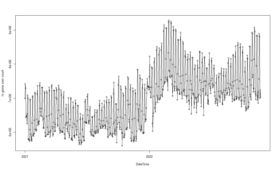
The data shows an upwards trend from 2021 to 2022.
But there are clearly two “layers” of the data, meaning that the maximum values and minimum values have similar trends if the data is viewed “separately”, but continuously, there is a clear seasonal trend.
Examination of the ACF, PACF, and EACF of the data:
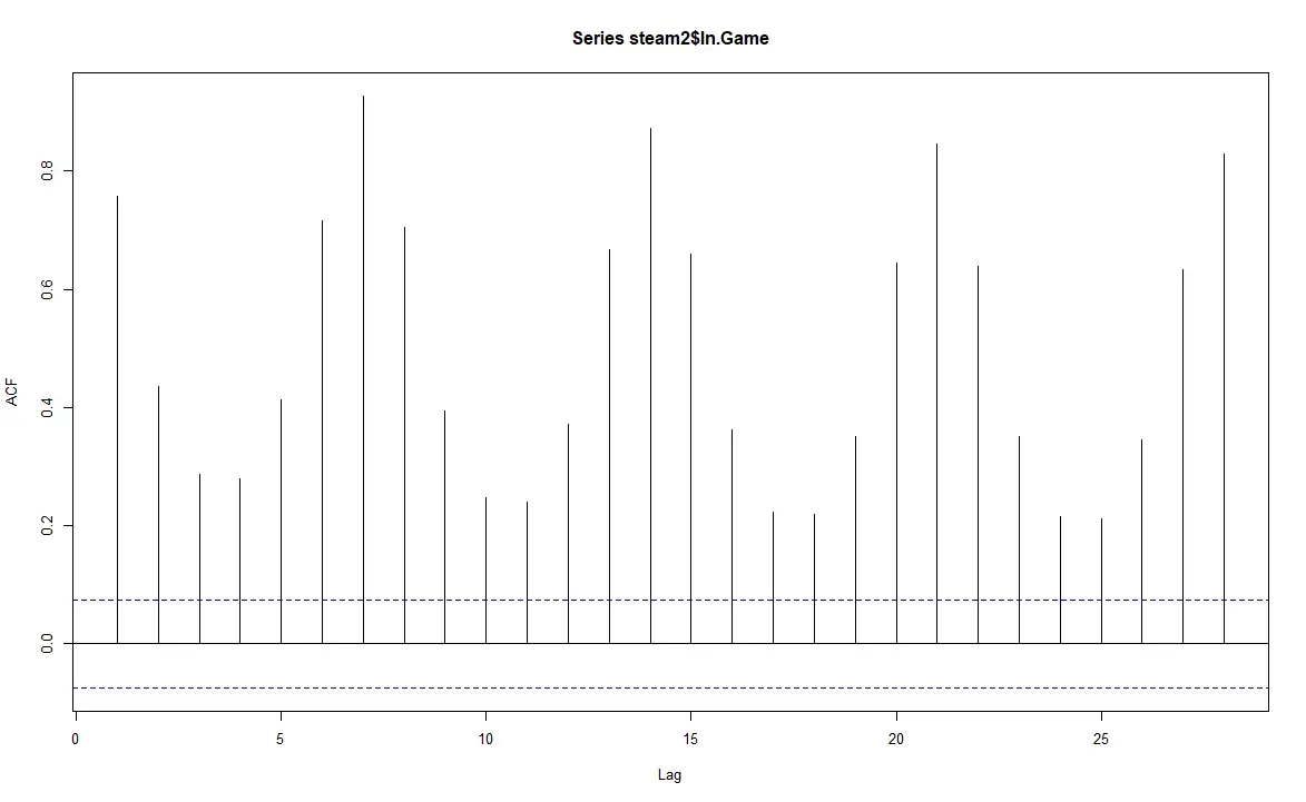
ACF(1.1)
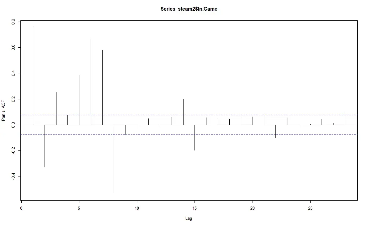
PACF(1.1)
From the ACF(1.1), we can see that the trend still exists, as the correlation reaches the max at around 0.8 for every lag7, and for lag2, lag3, lag4, and lag5.
There is a small negative correlation, meaning that the observation at lag n is largely positively determined by the observation at lag n-7, and somewhat negatively determined by observations at lag2, lag3, lag4, and lag5.
From the PACF(1.1), we can see that the PACF reduced to 0 after lag8, if we exclude the two observations in lag14 and lag15.
From the EACF, we can see it does not make much sense.
Since the pure stationary MA and AR models can be identified by studying their ACF and PACF, as the table of Box-Jenkins Identification Tables:

Box-Jenkins Table
By looking at the ACF for the series, we can see that the ACF does not decay exponentially, nor decays to zero after certain times, but instead there is a clear trend in the ACF for every 7 observations. For the PACF, we can see that the PACF dies out slowly exponentially, oscillating exponentially of a damped sine wave. Thus we conclude that the original series is neither a pure AR(p), MA(q), nor a ARMA(p,q).
Box-Jenkins Approach, Transform In.Game
The next step is to stationary transform the series. We can use a log change approach for a stationary transformation. We named the transformed set as steam.log.
> In.Game.log <- log(steam2$In.Game) - lag(log(steam2$In.Game))First, we plot the transformed data, and its ACF, PACF.
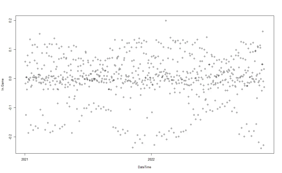
Transformed Plot
From the transformed plot, we can see that:
- there is still a layer of the different values.
- most observations lay in the middle of the plot, where the transformed in.game = 0.0, where there are two layers at around transformed in.game = +/- 0.2.
We need to examine the ACF and PACF.
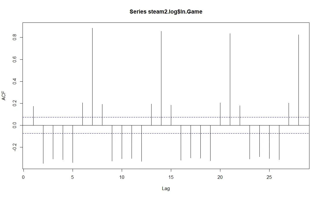
ACF(2.1)
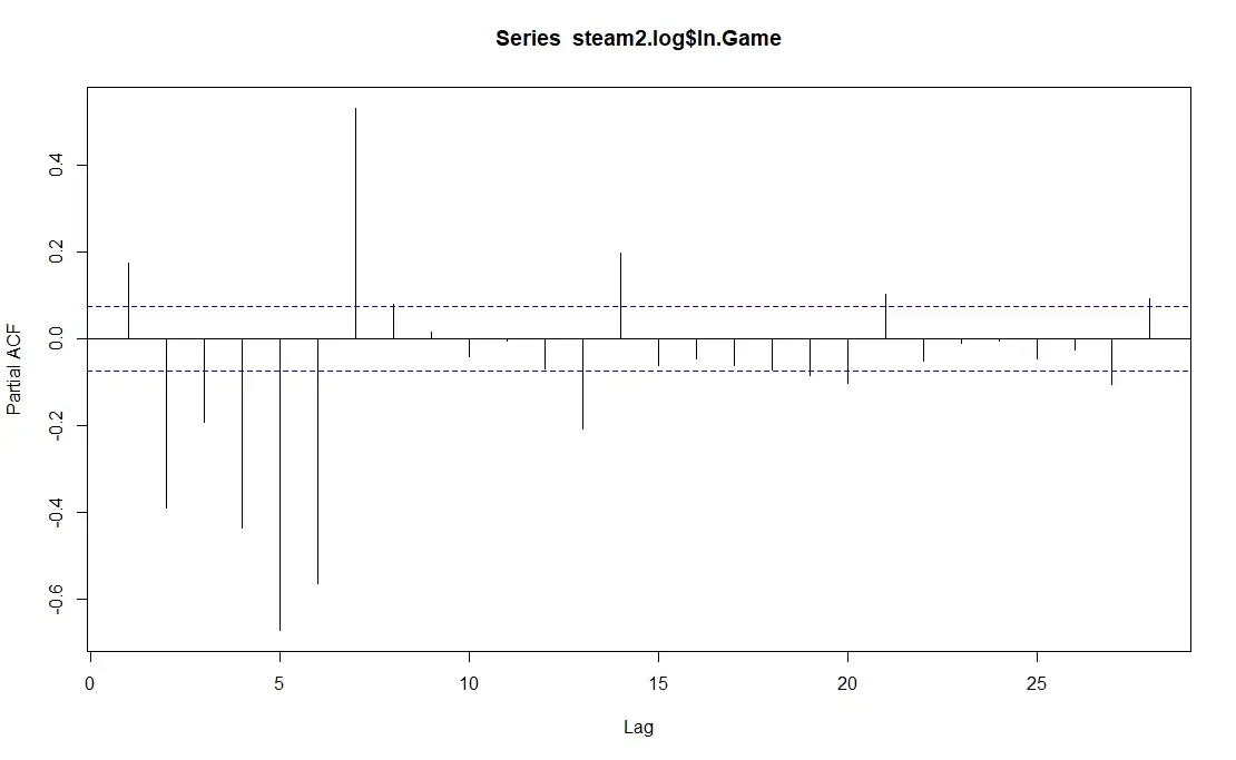
PACF(2.1)
From the ACF(2.1), we can see that the trend still exist, as the correlation reaches the max at around 0.8 for every lag7, and for lag2, lag3, lag4, and lag5, there is a small negative correlation, meaning that the observation at lag n is largely positively determined by the observation at lag n-7, and somewhat negatively determined by observations at lag2, lag3, lag4, and lag5.
The PACF(2.1) shows that there is indeed a diminishing return. We can see that the PACF reduced to 0 after lag8, if we exclude the two observations in lag13 and lag14.
Using the Box-Jenkins method, we can conclude that the series is neither a pure AR(p) or MA(q), nor a ARMA(p,q) model, by referring to the Box-Jenkins identification of MA or AR models table.
Dynamics Method (See Appendix for the Output Plot)
Using the dynamics method, start with assuming the series is an ARMA(p,q), consider all special cases for theta or phi equals 0.
Given the following outputs from the dynamic method, we could see that when trying to fit AR(1), phi_1 close to when but the log likelihood is a small number, while we could continue to examine the details in Dynamics Method, we have our conclusions of the series is neither pure MA(q), AR(p), nor ARMA(p,q) from the previous Box-Jenkins method.
We could save time and, rather, consider the clear seasonality of the series instead.
3.5 Seasonality
There is also a possibility that a multiplicative seasonal ARMA model may be better for our data. One hypothesis we could make is that there is a seasonal trend per seven days. After the first difference. The general upward trend has now disappeared.
There is a clear seasonal trend based on the ACF.
m1.steam <- arima(steam2$In.Game, order=c(2,1,2),seasonal=list(order=c(0,1,1), period=7))
Seaonal Model
Checking the histogram for standard error residuals, QQ plot for normality, and the ACF.
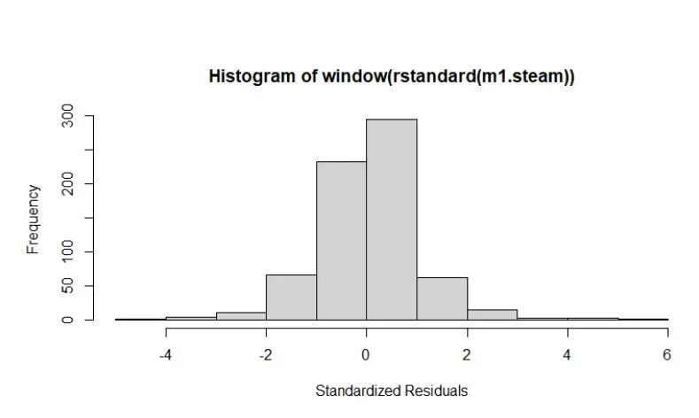
Standard Error for Residuals
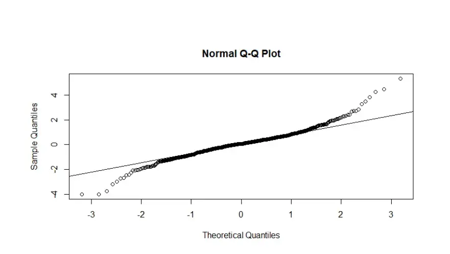
Normal QQ Plot
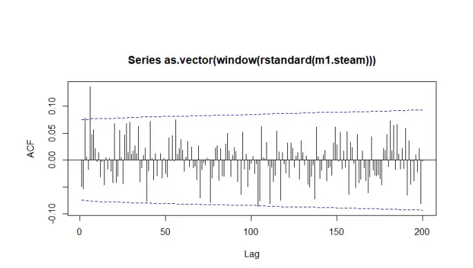
ACF
Acf for the seasonal model, clear that no data lay out side +- 2 sd.
Forecasting
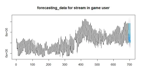
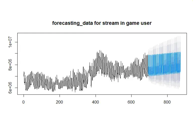
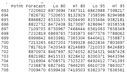
Based on the seasonal ARIMA model we get, we could do a forecasting of the number of active players in the future.
Here, we predict the next two weeks of player counts. Compared to the last observation of 7,023,597 players, we expect the player capacity for the next two weeks to be an estimated 9,487,428 in-game active players.
04 Concluding Remarks
In the end, we decided on the seasonal ARIMA model. Since the observations are on a daily basis, it’s clear that we can see a weekly pattern from the ACF. Thus, we chose an ARIMA(2,1,2) with seasonal (0,1,1) and a period of 7 units of time. This model can help the Steam company to predict possible player counts during the holidays so that they can be prepared to handle the sudden shock of in-game active players
Appendix
Reading Data into R
>library(dplyr)
>steam.raw <- read.csv("chart.csv", header = T)
>glimpse(steam.raw)
Preporcesssing
//Get the ratio of missing values for each variable
> colMeans(is.na(steam))
// Remove unnecessary variables
> steam.raw$Flags <- NULL
// Format DateTime observations to remove unreported Time
> steam.raw$DateTime <- as.Date(steam.raw$DateTime)
// Trim all records before 2020-01-01, store the trimmed data into steam2
n <- nrow(steam.raw)
idx <- match(as.Date("2020-01-01"), as.Date(steam.raw[,"DateTime"]))
steam2 <- steam.raw[idx:n,]
//Make sure the cleaned time series is continuous.
colMeans(is.na(steam2))
Forecasting
>forecastData <- forecast(m1.steam,14)
>plot(forecastData, main='tempView')
Forecast data
Plot
